
A tutorial introduction to using the PyTOPKAPI model is provided by way of an example simulation, set-up for the Liebenbergsvlei catchment in central South Africa. The tutorial materials for the example can be separately downloaded at http://github.com/sahg/PyTOPKAPI/downloads.
The example consists of a simulation of 42 days (lasting from 15/03/2000 to 26/04/2000) over a sub-catchment (3563 km2, defined by the flow station 2 in Figure 1 – station labelled C8H020) of the Liebenbergsvlei catchment. The simulations will be achieved at a 6-hour time-step at a spatial resolution of 1 km.
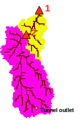
Figure 1: The Liebenbergsvlei catchment (delimited by the flow station 1) and the simulated sub-catchment in pink (delimited by the flow station 2).
In the directory TOPKAPI_Example/ is a directory called run_the_model/ that contains one file (TOPKAPI.ini) and two sub-directories (forcing_variables/ and parameter_files/).
In the directory forcing_variables/ are 3 files:
rainfield.h5 and ET.h5: these two files are respectively the rain fields and the evapotranspiration fields. The files are compressed binary files in a HDF5 format. The file structure can be easily seen (Figure 2) with the interface software HDF_Explorer provided in the directory Software_package. The file rainfields.h5 and ET.h5 are both composed of 1 group called sample_event. For the file rainfields.h5 the group contains one table called rainfall. For the file ET.h5 the group contains two tables called ETr and ETo, being respectively the reference crop evapotranspiration and the free surface reference evapotranspiration. In the tables rainfall, ETr and ETo the columns are the cells and the lines are the time steps.
external_lesotho_flows.dat: this file contains the external flows coming from Lesotho via the inter-basin transfer tunnel whose outlet is located at the Southern part of the catchment (see Figure 1). It is a simple 6 columns format in an ASCII format file containing the date (year, month, day, hour, minute) and the discharge at the outlet of the tunnel in m3/s (Figure 3).
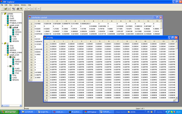
Figure 2: Forcing variable file rainfields.h5 and ET.h5 visualized with the software HDF_Explorer.
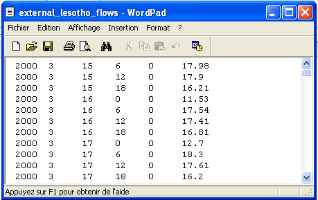
Figure 3: File external_lesotho_flows.dat : a simple column ASCII format containing the external flows coming in the catchment from the Lesotho by a tunnel.
The directory parameter_files/ contains the two parameter files required by the TOPKAPI model:
global_param.dat: it is an ASCII file containing all the parameters that are constant in the model. In the first line are the names of the variables. The values of the variables are reported in the second line (Figure 4).
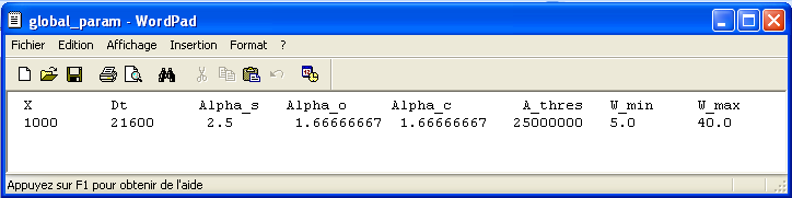
Figure 4: File global_param.dat: an ASCII file containing all the parameters that are constant for a given catchment.
From left to right in the file the reported parameters are:
 is the lateral dimension of the grid-cell (in
  ).
).
 is the time step of the model (in s)
 is a dimensionless pore-size distribution parameter
(Brooks and Corey, 1964)
is a dimensionless pore-size distribution parameter
(Brooks and Corey, 1964)
 and
and  are the well known power
coefficient equal to 5/3 originating from Manning’s equation.
are the well known power
coefficient equal to 5/3 originating from Manning’s equation.
 is the area over which a cell is considered to
initiate a river channel (in
is the area over which a cell is considered to
initiate a river channel (in  )
)
 is the minimum width of channel (in m)
 is the maximum width of channel (in m)
cell_param.dat: it is an ASCII file containing all the parameters that are spatially variable in the model. It is composed of 17 columns corresponding to 17 parameters (see Figure 5). Each line is a catchment cell, thus for our example (catchment area of 3563 km2 at a resolution of 1km2) the file is composed of 3563 lines.
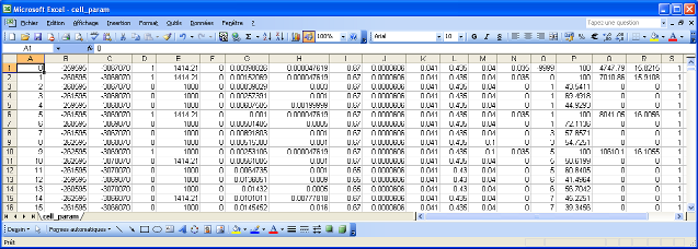
Figure 5: File cell_param.dat: an ASCII file containing all the parameters that are spatially variable in the model.
From left to right in the file the parameters are (note that the parameters are not labelled inside the file, but we identify them here by their column labels in the Excel list in Figure 5):
 equal to 1 if the cell is a channel cell, 0
otherwise.
equal to 1 if the cell is a channel cell, 0
otherwise. is the length of the channel cell (in m)
 the tangent of the ground slope angle

 the tangent of the channel slope angle

 the soil depth (in )
 the saturated hydraulic conductivity (in
  )
) the residual soil moisture content
 the saturated soil moisture content
 the Manning’s roughness coefficient for overland flows
 the Manning’s roughness coefficient for the channel
flows
the Manning’s roughness coefficient for the channel
flows the initial saturation of the soil reservoir (in
%)
the initial saturation of the soil reservoir (in
%) the initial water content of the overland
reservoir (in
the initial water content of the overland
reservoir (in  )
) the initial discharge in the channel (in
 )
) the crop coefficient
TOPKAPI.ini (in the directory run_the_model) is the input file (text file) required to run the model. It contains 6 main labels ([input_files], [output_files], [groups], [external_flow], [numerical_options] and [calib_params], see Figure 6).
In [input_files] are reported all the parameter and forcing files required by the model (labelled as file_global_param, file_cell_param, file_rain, file_ET).
In [output_files] is reported file_out an HDF format file in which will be written the simulation results.
In [groups] is reported the name of the group considered in the forcing HDF files.
In [external_flow] are reported: a Boolean parameter called external_flow, which is True when external flows are coming into the catchment, False otherwise; the coordinates Xexternal_flow and Yexternal_flow of the point where the flows come in; file_Qexternal_flow the file containing the discharge series of external flows.
In [numerical_options] are reported three variable solve_s, solve_o, solve_c, which take the value 1 to solve the ODE of respectively the soil, overland and channel reservoir by using a combination between the Quasi Analytical Solution and the Runge Kutta Fehlberg methods, the value 0 is set when only the Runge Kutta Felhberg method is to be used.
In [calib_params] are reported the four multiplying factors fac_L, fac_Ks, fac_n_o and fac_n_c that are applied on the a priori estimated parameters L, Ks, n_o and n_c. The factors proposed in the example come from the calibration procedure realized on the Liebenbergsvlei catchment.
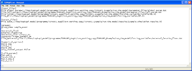
Figure 6: TOPKAPI.ini is the input file (text file) required to run the model.
Open the directory TOPKAPI_Example/. It contains three sub-directories that correspond to the three steps of the process presented in the introduction (create_the_parameter_files, run_the_model and analyse_the_results). In addition there is a small file called run_example.py which is a Python command file, designed to run the tutorial in one action. The following discussion takes the reader step-by-step through the process to provide a better idea of the structure of the processes.
Open a command shell for Python. If you installed IPython on Windows then click on Start-All programs-IPython.
Type the following commands in the Python Shell (the shell commands are hereafter highlighted in grey):
# import the package pytopkapi
import pytopkapi
# navigate to the TOPKAPI_Example directory
cd C:\ … \TOPKAPI_Example
# Run the model using the supplied configuration
pytopkapi.model.run('run_the_model/TOPKAPI.ini')
The simulation starts and will last around 3 to 5 minutes depending on your machine. Some comments are written and the number of time steps (to 169 of 6 hours each) scrolls followed by ‘* THE END *’. Leave the iPython window open - we will use it shortly.
At the end of the simulation, a folder results should have been created in the run_the_model folder, containing an HDF5 file called Example_simulation_results.h5; to open it you will have to associate the file (if it’s the first *.h5 file you’ve opened) with HDF_Explorer. This file is composed of three groups: Channel, Overland and Soil. The group Channel contains the table Qc_out that is the channel flow of each cell (in m3/s) [to view a file’s content, double click on the little green square under the yellow label in the left panel of the window - see Figure 7.] The group Overland contains the table V_o that is the volume of the overland reservoir (in m3). The group Soil contains the table V_s that is the volume of the soil reservoir (in m3). For the three tables Qc_out, V_o and V_s, the 3563 columns are the cells and the 170 rows are the time steps.
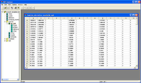
Figure 7: File Example_simulation_results.h5 in which are written the simulation results.
The analysis of the simulations consist of two simple modules that allow the user to (i) plot the rainfall-runoff graphic (simulated and observed discharge and rainfall on the same graph), module called plot_Qsim_Qobs_Rain and (ii) plot maps of soil moisture over the catchment, module called plot_soil_moisture_maps.
a.Plot of the rainfall runoff graphic
The directory TOPKAPI_Example/ contains a directory called analyse_the_results/. In analyse_the_results/ the results are three files amongst them plot_Qsim_Qobs_Rain.ini and C8H020_6h_Obs_Example.dat.
C8H020_6h_Obs_Example.dat is an ASCII file in a column format
containing the date and the value of discharge (in ) at
the flow station at the outlet of the simulated catchment (station
labelled 2 in Figure 1).
plot_Qsim_Qobs_Rain.ini is the input file to the module plot_Qsim_Qobs_Rain. As reported on Figure 8, it contains three items [files], [groups] and [flags]. In [files] are reported all the input files required by the program as well as the output file which must be ended by a typical picture format (*.png, *.jpg, …). In [groups] is reported the name of the group to look in the result of simulation file. With [flags] are associated three Boolean that correspond to different options in the graphic: Qobs must be True to plot the observed discharges, Pobs must be True to plot the observed rainfall and nash must be True to write on the graph the Nash efficiency comparing observed and simulated discharges.
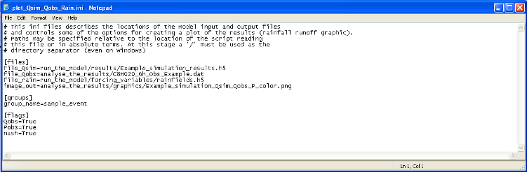
Figure 8: File plot_Qsim_Qobs_Rain.ini, input file to the module plot_Qsim_Qobs_Rain.
In the Python shell, import the module plot_Qsim_Qobs_Rain
ln [4]: from pytopkapi.results_analysis import plot_Qsim_Qobs_Rain
# Create a plot of the simulated and observed discharge records
ln [5]: plot_Qsim_Qobs_Rain.run('analyse_the_results/plot_Qsim_Qobs_Rain.ini')
This should create an image file called Example_simulation_Qsim_Qobs_P_color.png (Figure 9) in the directory TOPKAPI_Example/analyse_the_results/graphics.
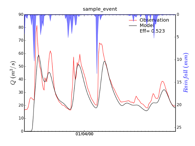
Figure 9: The image file Example_simulation_Qsim_Qobs_P_color.png.
In the directory TOPKAPI_Example/analyse_the_results., the last of three files is plot_soil_moisture_maps.ini. As reported on Figure 10, it contains three items [files], [paths] [calib_params] and [flags].
[files] contains all the input files required by the program meaning the two parameter files of the TOPKAPI model (cell and global), and the result of simulation file.
In [paths] is reported the path in which the maps will be saved.
In [calib_params] are reported the four multiplying factors fac_L, fac_Ks, fac_n_o and fac_n_c that were applied in the TOPKAPI simulation (see Section 2.1).
In [flags] are reported several variables required by the program:
the maps will be plotted from the time step t1 to the time step t2,
the first time step at the beginning of the simulation being 0. Four
choices (1,2,3 or 4) are available for the variable called variable
which determines which variable is to be plotted among (1) the soil
moisture content i.e. the volume of the soil reservoir in ,
(2) the water content of the overland i.e. the volume of the overland
reservoir in , (3) the saturation binary index which is 1
for the saturated cells, 0 otherwise, (4) the soil water index
i.e. the saturation rate of the cell in %.
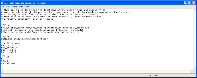
Figure 10: File plot_Qsim_Qobs_Rain.ini, input file to the module plot_Qsim_Qobs_Rain.
This should create 20 pictures called field_SWI_0001.png,…, field_SWI_0020.png in the directory TOPKAPI_Example/analyse_the_results/maps. One of them is plotted on Figure 11.
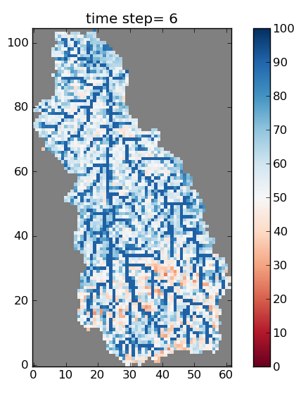
Figure 11: One of the 20 soil moisture maps (here the Soil Water Index is plotted) as a result of the program plot_soil_moisture_maps.
Nota Bene
Alternatively the entire process (from running the model to analysing the results) can be produced by running the script contained in the file run_example.py located in TOPKAPI_Example/.
import pytopkapi

# run a model simulation using the configuration in TOPKAPI.ini
pytopkapi.run('run_the_model/TOPKAPI.ini')

# plot the simulation results (rainfall-runoff graphics) using the
# config in plot_Qsim_Qobs_Rain.ini
from pytopkapi.results_analysis import plot_Qsim_Qobs_Rain

plot_Qsim_Qobs_Rain.run('analyse_the_results/plot_Qsim_Qobs_Rain.ini')


# plot the simulation results (soil moisture maps) using the config in
# plot_soil_moisture_maps.ini
from pytopkapi.results_analysis import plot_soil_moisture_maps

plot_soil_moisture_maps.run('analyse_the_results/plot_soil_moisture_maps.ini')
 Copyright 2008-2010, Theo Vischel, Scott Sinclair & Geoff Pegram
Last updated on Nov 01, 2010
| Created using Sphinx